The PID controller, explained simply
How a robot joint reaches exactly the angle you ask for: feedback, the three letters of PID as present, past and future, what each one does on a real move, how to tune the gains, and the three traps to avoid. With pictures from a simulation and short Python and Arduino code.
Ask a robot arm to move its elbow to 60°. The motor spins, the arm swings, and it stops at 60°. Not 57°, not 63°, and it stays there even though gravity keeps pulling the arm down. How?
Almost certainly, a PID controller did it. It is a few lines of code, it is about a hundred years old, and it runs inside most of the machines around you: robot joints, drones, 3D printers, cruise control, ovens, even coffee makers. Once you understand it, you will start seeing it everywhere.
$$ \underbrace{\text{Target}}_{\text{where I want to be}} \;-\; \underbrace{\text{Measurement}}_{\text{where I am}} \;=\; \underbrace{\text{Error}}_{\text{how wrong I am}} \;\rightarrow\; \text{PID} \;\rightarrow\; \text{Motor} \;\rightarrow\; \text{measure again} $$
An analogy. Think of adjusting the water in the shower. You feel it (measure), notice it is too cold (error), turn the handle toward hot (act), and feel again. A big error gets a big turn, a small error a small nudge. You are already a feedback controller. PID is just that habit written down carefully.
1. Why a robot needs feedback
The simplest way to drive a motor is to send it a fixed amount of power and hope. This is open-loop control. A toaster works this way: it heats for two minutes whether the bread is thin or thick, fresh or frozen. Sometimes you get charcoal.
A robot joint cannot work like a toaster. The load changes, the gears are stiffer on a cold morning, and gravity pulls differently in every pose. So instead of hoping, the controller measures the result and corrects the action, again and again. That is closed-loop control, or simply feedback.
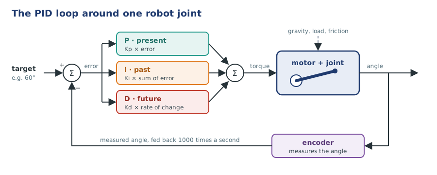
Every feedback loop has the same five parts:
| Part | What it is | On a robot joint |
|---|---|---|
| Target (setpoint) | The value you want | 60° |
| Sensor | Measures what you actually have | Encoder on the motor shaft |
| Error | Target minus measurement | 60° − 52° = 8° |
| Controller | Turns the error into a command | The PID code |
| Actuator | Carries out the command | Motor and driver |
The beautiful part: the controller does not need to know how heavy the arm is or how stiff the gears are. It only keeps pushing in the direction that makes the error smaller. Feedback forgives ignorance.
2. Three questions about one error
How should the controller turn an error into a command? PID answers by asking three simple questions about the same error, one about the present, one about the past and one about the future. (The idea goes back to 1922, when the engineer Nicolas Minorsky studied how experienced helmsmen steered ships.)
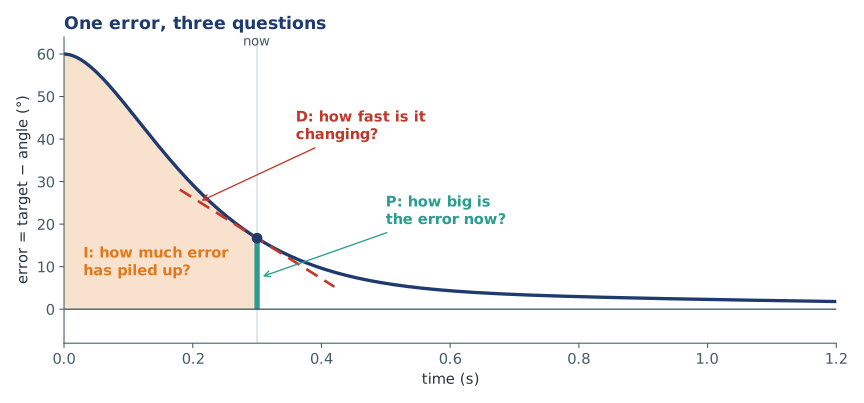
Imagine you are driving and want to hold exactly 100 km/h.
P is for proportional: how big is the error right now? The further you are below 100, the harder you press the pedal. At 70 km/h you push firmly; at 98 you barely touch it. P does most of the work. But it has a weakness: as you get close, the push fades away. Going uphill, you may settle at 96 km/h and never quite get there.
I is for integral: how much error has piled up? You notice you have been a bit slow for a while. That lingering gap bothers you more the longer it lasts, so you slowly press harder until it is gone. I adds up the past error. It is the one that removes small, stubborn gaps.
D is for derivative: how fast is the error changing? You see the speedometer climbing quickly toward 100. If you keep your foot down, you will shoot past. So you ease off before you arrive. D looks at the trend and brakes early. It stops overshoot and calms things down.
The controller simply adds the three answers:
$$ u(t) \;=\; \underbrace{K_p\, e(t)}_{\text{present}} \;+\; \underbrace{K_i \int_0^t e(\tau)\,d\tau}_{\text{past}} \;+\; \underbrace{K_d\, \frac{de(t)}{dt}}_{\text{future}} $$
Here \(e\) is the error, \(u\) is the command to the motor, and the three numbers \(K_p, K_i, K_d\) (the gains) decide how much each question counts. Inside a computer, time comes in small steps \(\Delta t\) (say 1 ms), and the formula becomes plain arithmetic:
$$ u_k = K_p\, e_k \;+\; K_i \sum_{j=0}^{k} e_j\,\Delta t \;+\; K_d\, \frac{e_k - e_{k-1}}{\Delta t} $$
Multiply, add up, subtract. That is all.
3. Watching it work on a robot joint
Let us try it on a simulated robot joint: a motor turning an arm link. The motor can give at most 5 N·m of torque, and gravity pulls on the arm with 0.6 N·m (we keep it constant to make things simple). The task: move from 0° to 60°. We add the letters one at a time.
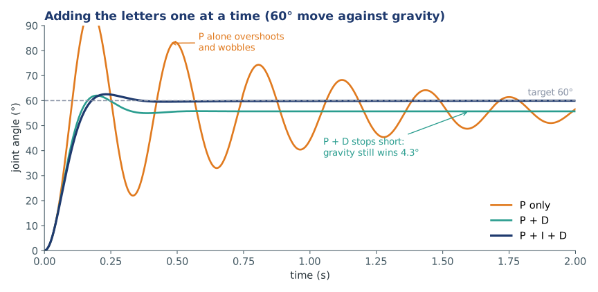
| Controller | Gains \(K_p, K_i, K_d\) | Overshoot | Final angle | Settled (within ±2 %) |
|---|---|---|---|---|
| P only | 8, 0, 0 | 36.7° (61 %) | 55.7° | never: keeps wobbling, stops short |
| P + D | 8, 0, 0.4 | 2.0° | 55.7° | never: calm, but stops short |
| P + I + D | 8, 10, 0.5 | 2.5° | 60.0° | 0.30 s |
P only gets there fast but swings past the target and wobbles for seconds. Even when the wobbling dies out, it stops short.
Why does it stop short? To hold the arm still, the motor must push back against gravity with 0.6 N·m. With only P, the motor only pushes when there is an error, so some error has to remain:
$$ K_p \cdot e = 0.6 \;\;\Rightarrow\;\; e = \frac{0.6}{8} = 0.075 \text{ rad} = 4.3^\circ $$
That is exactly the gap in the plot: 60° − 4.3° = 55.7°. A bigger \(K_p\) shrinks the gap but makes the wobbling worse. P alone can never close it completely.
P + D brakes before the target, so the wobbling is gone. But D only reacts to change, and a still arm is not changing, so the 4.3° gap stays.
P + I + D is the full controller. The I term keeps adding up the gap until it pushes hard enough to cancel gravity, and the arm lands on 60.0° in 0.3 s.
Who does what during the move
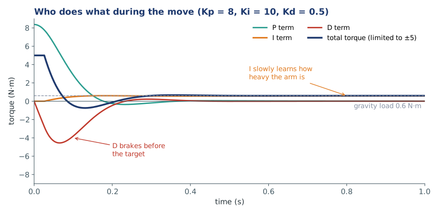
Looking at each term separately tells the whole story:
- At the start the error is large, so P asks for 8.4 N·m. The motor can only give 5, so it runs flat out.
- As the arm speeds up, D pulls in the opposite direction. It is braking before the arm reaches the target.
- I grows slowly and settles at exactly 0.6 N·m, the weight of the arm. Nobody told the controller how heavy the arm is. The I term learned it from the error.
- At the end, P and D fall to zero (no error, no motion), and only I is left, holding the arm up against gravity.
4. Tuning: timid, aggressive or just right
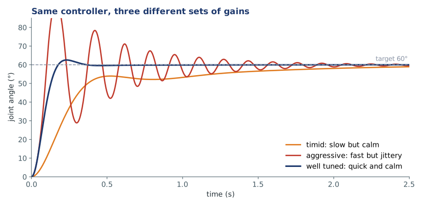
The same controller behaves very differently with different gains. Choosing them is called tuning.
| Tuning | Gains \(K_p, K_i, K_d\) | Reaches 90 % of the move | Overshoot | Settled (±2 %) |
|---|---|---|---|---|
| Timid | 1.5, 1.5, 0.15 | 1.08 s | none | 2.42 s |
| Aggressive | 30, 40, 0.05 | 0.10 s | 33.3° (56 %) | 1.86 s |
| Well tuned | 8, 10, 0.5 | 0.14 s | 2.5° (4 %) | 0.30 s |
Notice that the aggressive controller is fast to arrive but slow to settle. Speed is not about pushing hard; it is about pushing at the right moments.
What each gain does
| Turn up… | Speed | Overshoot | Leftover error | Watch out for |
|---|---|---|---|---|
| \(K_p\) | Faster | More | Smaller | Wobbling, then shaking |
| \(K_i\) | Slightly faster | More | Removed | Slow swings, windup |
| \(K_d\) | About the same | Less | No effect | Amplified sensor noise |
A simple tuning recipe
- Set \(K_i = 0\) and \(K_d = 0\). Raise \(K_p\) until the joint moves briskly and overshoots a little.
- Raise \(K_d\) until the overshoot is gone or small. If the motor starts buzzing, you went too far.
- Raise \(K_i\) slowly until the leftover error disappears in a reasonable time. Stop before slow swings appear.
- Test with the real load, small and large moves, and go back to step 1 if needed.
There are formal methods too (Ziegler–Nichols, model-based tuning, auto-tuners), but this hands-on recipe is how most people tune their first motor.
5. Three traps (and their simple fixes)
Trap 1: integral windup
When the motor is already giving everything it has, the error is still large, and I keeps adding it up. By the time the arm arrives, I has grown huge and pushes it far past the target.
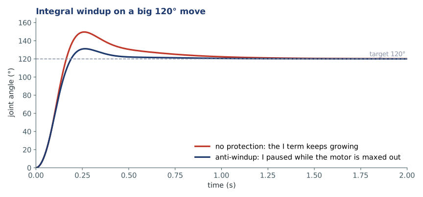
On a 120° move with \(K_i = 20\), the unprotected controller overshoots by 29.7°; with anti-windup only 11.2°, and it settles twice as fast (0.48 s instead of 0.99 s). The fix is one line: stop adding to the integral while the motor is maxed out.
Trap 2: derivative kick
If the target jumps from 0° to 60° in an instant, the error jumps too, and its "rate of change" is enormous for one step. D sends a violent spike to the motor. The fix: compute D from the measurement instead of the error. When the target is constant they are the same; when the target jumps, the measurement does not.
Trap 3: noise and delay
D looks at changes, so it amplifies sensor noise: a jittery encoder becomes a buzzing motor. Filter the measurement a little, or keep \(K_d\) modest. Delay is the other enemy: if the measurement arrives late, the controller reacts to the past and overshoots. This is why motor loops run fast, typically 1 to 10 kHz.
6. Code: a complete PID controller in Python
This is the whole controller, including both fixes from section 5:
class PID:
    def __init__(self, kp, ki, kd, out_min, out_max):
        self.kp, self.ki, self.kd = kp, ki, kd
        self.out_min, self.out_max = out_min, out_max
        self.integral = 0.0
        self.prev_measurement = None

    def update(self, target, measurement, dt):
        error = target - measurement                                  # P: the present

        if self.prev_measurement is None:
            rate = 0.0
        else:                                                         # D: the future
            rate = -(measurement - self.prev_measurement) / dt        # from measurement: no kick
        self.prev_measurement = measurement

        candidate = self.integral + error * dt                        # I: the past
        out = self.kp * error + self.ki * candidate + self.kd * rate
        if self.out_min < out < self.out_max:                         # anti-windup
            self.integral = candidate

        out = self.kp * error + self.ki * self.integral + self.kd * rate
        return max(self.out_min, min(self.out_max, out))              # respect the motor's limit
7. Code: try it on a simulated joint
No hardware needed. The joint obeys one line of physics: inertia × acceleration = motor torque − friction − gravity.
import math

J, friction, gravity = 0.02, 0.05, 0.6      # kg·m², N·m·s/rad, N·m
dt, target = 0.001, math.radians(60)        # 1 kHz loop, 60° target

pid = PID(kp=8, ki=10, kd=0.5, out_min=-5, out_max=5)
angle = speed = 0.0
for step in range(2000):                    # two seconds
    torque = pid.update(target, angle, dt)
    accel = (torque - friction * speed - gravity) / J
    speed += accel * dt
    angle += speed * dt
    if step % 200 == 0:
        print(f"t = {step * dt:.1f} s   angle = {math.degrees(angle):5.1f}°   torque = {torque:5.2f} N·m")

print(f"final: {math.degrees(angle):.2f}°, I term = {pid.ki * pid.integral:.2f} N·m (the arm's weight)")
Change the gains and watch what happens: set ki=0 to see the 4.3° gap appear, or kd=0 to see the overshoot. The simulation behind every figure in this post is pid_joint_sim.py.
8. Code: the same controller on an Arduino
For a DC motor with a quadrature encoder and a driver with direction and PWM pins (for example an L298N):
const int ENC_A = 2, ENC_B = 3;          // encoder channels (pin 2 has an interrupt)
const int PWM_PIN = 9, DIR_PIN = 8;      // motor driver
const float COUNTS_PER_REV = 1440.0;     // encoder pulses per rev × gear ratio

const float KP = 2.0, KI = 0.5, KD = 0.05;   // starting values: tune for your motor
const float OUT_LIMIT = 255.0;               // full PWM
const unsigned long PERIOD_US = 1000;        // 1 kHz loop

volatile long counts = 0;
float target = 90.0;                     // degrees
float integral = 0.0, prevAngle = 0.0;
unsigned long last = 0;

void onEncoder() { counts += digitalRead(ENC_B) ? 1 : -1; }

float readAngle() {
  noInterrupts(); long c = counts; interrupts();
  return c * 360.0 / COUNTS_PER_REV;
}

void setMotor(float cmd) {
  digitalWrite(DIR_PIN, cmd >= 0 ? HIGH : LOW);
  analogWrite(PWM_PIN, (int)fabs(cmd));
}

void setup() {
  pinMode(ENC_A, INPUT_PULLUP);
  pinMode(ENC_B, INPUT_PULLUP);
  pinMode(PWM_PIN, OUTPUT);
  pinMode(DIR_PIN, OUTPUT);
  attachInterrupt(digitalPinToInterrupt(ENC_A), onEncoder, RISING);
  prevAngle = readAngle();
  last = micros();
}

void loop() {
  unsigned long now = micros();
  if (now - last < PERIOD_US) return;    // run at a steady rate
  float dt = (now - last) * 1e-6;
  last = now;

  float angle = readAngle();
  float error = target - angle;
  float rate = -(angle - prevAngle) / dt;            // D from the measurement
  prevAngle = angle;

  float out = KP * error + KI * (integral + error * dt) + KD * rate;
  if (out > -OUT_LIMIT && out < OUT_LIMIT) integral += error * dt;   // anti-windup
  out = KP * error + KI * integral + KD * rate;
  setMotor(constrain(out, -OUT_LIMIT, OUT_LIMIT));
}
The gains here are in "PWM per degree", not N·m per radian, so they are different numbers from the simulation. Start low and follow the tuning recipe in section 4. If the motor runs away instead of settling, swap the motor wires or the encoder channels: the feedback sign is reversed.
Common problems and fixes
| Problem | Likely cause | Fix |
|---|---|---|
| Joint stops a few degrees short | No I term, or \(K_i\) too small | Add or raise \(K_i\) |
| Overshoots and wobbles | \(K_p\) too high, \(K_d\) too low | Lower \(K_p\) or raise \(K_d\) |
| Big overshoot only on large moves | Integral windup | Add anti-windup |
| Motor buzzes or whines at rest | \(K_d\) amplifying encoder noise | Lower \(K_d\), filter the measurement |
| Violent jerk when the target changes | Derivative kick | Take D from the measurement |
| Slow, lazy swings that take seconds | \(K_i\) too high | Lower \(K_i\) |
| Motor runs away at full speed | Feedback sign reversed | Swap motor wires or encoder channels |
| Works in simulation, wobbles on hardware | Loop too slow or delayed | Run the loop faster and at a steady rate |
The short version
- Feedback means measure, compare with the target, correct, repeat. It works without knowing the machine exactly.
- P looks at the present error and does most of the work, but leaves a gap under a steady load.
- I adds up past error and removes that gap. It learns, for example, how heavy the arm is.
- D watches how fast the error changes and brakes early, preventing overshoot.
- Tuning balances the three: fast but calm. Raise \(K_p\), then \(K_d\), then \(K_i\).
- Protect against windup, derivative kick and noise, and run the loop fast.
Further reading
- Improving the Beginner's PID, Brett Beauregard: the classic step-by-step guide to the details in section 5
- Arduino PID Library, the library that grew out of that series
- Karl J. Åström and Richard M. Murray, Feedback Systems: An Introduction for Scientists and Engineers: the next step when you want the theory
- On this site: Robot kinematics and dynamics for where the target angles come from, and Arduino development for wiring up motors and encoders
Try it yourself
- Be a PID controller. Next time you shower, notice your first big turn (P), easing off as it gets warm (D) and the final small nudge when it stays a bit cool (I). Notice the delay between turning and feeling: delay is what makes control hard.
- In the simulation from section 7, set
gravity = 1.2. How big is the gap withki=0? Check your answer with \(e = 1.2 / K_p\). - Find the smallest \(K_d\) that keeps the overshoot under 5 % with \(K_p = 8\).
- When you ride a bicycle, are you mostly using P, I or D? What happens to a beginner who uses too much P?