Dynamic Covariance Scaling, explained simply
How a SLAM system survives one wrong 'I've been here before': pose graphs, loop closures, why a single false loop closure can wreck a map, and how Dynamic Covariance Scaling (DCS) turns its volume down. A robot with a RealSense camera drives down a corridor to a lab and back, with every number from a runnable simulation.
Drive a robot 20 m down a corridor to the lab and back. Its camera sees desks, chairs, doors. Somewhere on the way back it recognises a spot and says: "I have been here before." If that is true, the map gets better. If it is false, the map can end up worse than if the robot had done nothing at all.
In the simulation below, one wrong loop closure out of four pushed the average trajectory error from 0.27 m (no loop closures at all) to 0.34 m. Adding information made the answer worse. The fix is a single line of arithmetic, and it is called Dynamic Covariance Scaling (DCS).
$$ \text{constraint} \;\rightarrow\; \underbrace{\chi^2}_{\text{how much it disagrees}} \;\rightarrow\; \underbrace{s = \min\!\left(1,\; \frac{2\Phi}{\Phi + \chi^2}\right)}_{\text{how much to trust it}} \;\rightarrow\; \text{optimize again} $$
An analogy. Picture a mixing desk. Every measurement is a channel, and the optimizer listens to the sum. Most channels say roughly the same thing. One channel is shouting something completely different. You could unplug it (that is outlier rejection), but you might be unplugging a channel that is right. DCS does something gentler: it turns that channel's volume down, further the louder and more inconsistent it is, and keeps listening.
1. The robot and the corridor
The robot has an Intel RealSense RGB-D camera on its head. It starts at the beginning of a 20 m corridor lined with desks and chairs, drives to the lab at the far end (desks, tables, PCs, other robots, people) and drives back to where it started.
Everything in this post comes from a small simulation of exactly that trip, so every number can be reproduced. The setup:
| Quantity | Value |
|---|---|
| Path | 20 m out, 20 m back, one pose every 1 m (41 poses) |
| Odometry noise | 2 cm per step |
| Odometry drift | a constant bias of about 1 cm per step, in the same direction on the way out and the way back |
| Loop-closure noise | 10 cm |
| Loop closures | 3 correct, 1 false |
The numbers describe a generic visual-inertial or RGB-D odometry that slowly drifts. They are not measurements from a specific RealSense model. The code is at the end.
2. How SLAM thinks: a chain and some shortcuts
Visual SLAM is usually split in two halves.
| Part | Job | On our robot |
|---|---|---|
| Front end | Turns images into measurements | Match features between frames, reject bad matches (for example with RANSAC), estimate how far the camera moved, recognise places it has seen before |
| Back end | Turns measurements into the best trajectory | Optimize a pose graph |
A pose graph is a very simple object. Every node is the robot's pose at one moment. Every edge is a measurement that says how two poses relate.
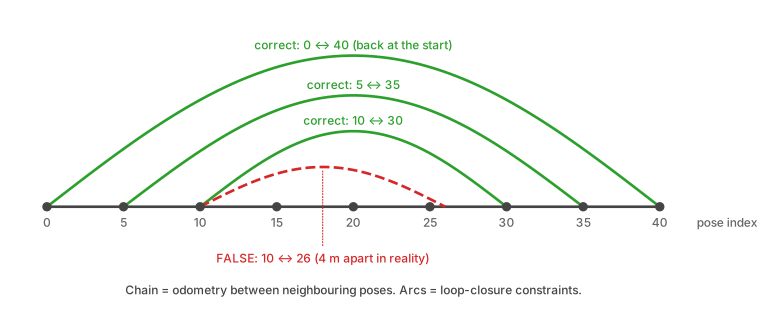
There are two kinds of edges:
- Odometry edges connect neighbouring poses: "I moved about 1 m forward." Each one is small and slightly wrong, and the errors add up. This is drift.
- Loop-closure edges connect poses far apart in time: "this is the same place as before." They are the only thing that can cancel drift, because they tie the end of the trip back to the start.
The optimizer finds the trajectory that disagrees least with all edges at once. Disagreement is measured by the residual \(r\), the gap between what an edge says and what the current trajectory implies, weighted by the edge's confidence:
$$ \min_{\mathbf{x}} \sum_i \mathbf{r}_i^\top\, \boldsymbol{\Omega}_i\, \mathbf{r}_i, \qquad \boldsymbol{\Omega}_i = \boldsymbol{\Sigma}_i^{-1} $$
\(\boldsymbol{\Sigma}_i\) is the covariance of edge \(i\): how uncertain it is. \(\boldsymbol{\Omega}_i\) is its inverse, the information: how much the optimizer should care. A confident edge (small covariance) pulls hard. A vague edge (large covariance) pulls gently.
Remember that last sentence. DCS is built entirely on it.
3. Drift, and what loop closures fix
Without loop closures the robot only has the chain. Because the odometry bias does not cancel when the robot turns around, the error keeps growing:
- about 0.2 m at the lab door,
- about 0.45 m back at the start (average over 300 random runs),
- average error along the whole trip, measured as RMSE: 0.27 m.
Now the robot comes back, recognises the start and adds a loop closure: "pose 40 is the same place as pose 0, up to 10 cm." Together with the other two correct loop closures, the optimizer can bend the whole chain back into shape. The RMSE drops to 0.11 m.
That is the dream scenario, with only correct loop closures.
4. The false loop closure
Corridors are repetitive. Desk rows look like desk rows, and one chair next to one door looks a lot like another chair next to another door. A place-recognition system compares how a view looks, not where it is.
Suppose the robot, at pose 26 on the way back (14 m from the start), sees a desk arrangement that looks just like the one at pose 10 (10 m from the start). It concludes: "same place."
The two poses are really 4 m apart. The loop-closure edge claims they are 0 m apart, and claims it with a 10 cm uncertainty. In the pose graph's eyes that is a disagreement of
$$ \chi^2 = \frac{(4\ \text{m})^2}{(0.10\ \text{m})^2} = 1600 $$
compared with a value around 1 or 2 for a loop closure that is correct. Yet the optimizer has been told this edge is precise, so it obeys it. The only way to satisfy "poses 10 and 26 coincide" is to squeeze the 16 poses between them together, and the squeeze drags everything after them.
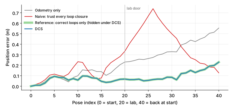
The red line is the naive optimizer. It does reduce the error near the end, but it creates a hump of about 0.7 m right where the false loop was added, and the average error over the whole trip is worse than odometry alone.
One more lesson from this plot. Look only at the final pose and the naive run (0.13 m) looks better than DCS (0.23 m) in this particular run. The distortion happened to push the last pose toward the right place. The trajectory as a whole is wrong almost everywhere else. Always judge a SLAM result by the whole trajectory, not by where it happens to end.
5. DCS: turn the volume down, in proportion to the disagreement
Dynamic Covariance Scaling (Agarwal, Tipaldi, Spinello, Stachniss and Burgard, 2013) looks at how much each loop closure disagrees with everything else and scales its covariance accordingly:
$$ s_i = \min\!\left(1,\; \frac{2\Phi}{\Phi + \chi_i^2}\right), \qquad \boldsymbol{\Omega}_i' = s_i^2\, \boldsymbol{\Omega}_i $$
Read the first formula from the outside in:
- If \(\chi_i^2 \le \Phi\), the constraint is plausible, \(s_i = 1\), and nothing changes.
- If \(\chi_i^2 > \Phi\), the scale \(s_i\) falls below 1. The larger the disagreement, the smaller the scale.
- The information is multiplied by \(s_i^2\), which is the same as multiplying the covariance by \(1/s_i^2\). The standard deviation grows by \(1/s_i\).
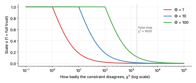
\(\Phi\) is the only knob. It sets where the curve starts bending: a smaller \(\Phi\) is more suspicious, a larger \(\Phi\) more trusting.
The optimizer then repeats the loop: solve, measure each constraint's \(\chi^2\) at the new solution, recompute the scales, solve again. Because \(s\) depends on the current estimate, it is "dynamic".
The numbers for our false loop
With \(\Phi = 10\), after the optimizer has settled:
| Loop closure | \(\chi^2\) at the solution | Scale \(s\) | Effective std dev |
|---|---|---|---|
| 0 ↔ 40 (correct) | 2.5 | 1.00 | 10 cm |
| 5 ↔ 35 (correct) | 2.5 | 1.00 | 10 cm |
| 10 ↔ 30 (correct) | 0.2 | 1.00 | 10 cm |
| 10 ↔ 26 (false) | 1,615 | 0.012 | about 8 m |
The false loop closure still exists. It still says "these two poses coincide". But its claimed precision went from 10 cm to roughly 8 m, which at a trajectory this size is a murmur, not a shout. The three correct loop closures never noticed.
6. Does it work? Numbers from 300 random runs
Each run draws new odometry and loop-closure noise. The table shows the mean over 300 runs. RMSE is the average position error over all 41 poses.
| Method | RMSE (m) | Error at the final pose (m) |
|---|---|---|
| Odometry only | 0.273 | 0.453 |
| Naive: trust every loop closure | 0.343 | 0.219 |
| DCS (\(\Phi = 10\)) | 0.107 | 0.147 |
| Reference: only the correct loops (cheating, it knows which one is false) | 0.107 | 0.145 |
DCS matches the cheating reference, even though it was never told which loop was false.
Choosing \(\Phi\)
\(\Phi\) is not free. Same 300 runs, \(\Phi\) varied:
| \(\Phi\) | RMSE (m) | Mean scale of the false loop | Mean scale of the correct loops |
|---|---|---|---|
| 1 | 0.244 | 0.001 | 0.34 |
| 3 | 0.143 | 0.004 | 0.86 |
| 10 | 0.107 | 0.012 | 1.00 |
| 100 | 0.104 | 0.117 | 1.00 |
| 1000 | 0.343 | 1.000 | 1.00 |
- \(\Phi\) too small (1): the optimizer is so suspicious that it also turns down the correct loop closures. Early on, the trajectory is still drifted, so even correct loops disagree with it. Result: most of the drift correction is lost and RMSE (0.244 m) ends up close to the odometry-only value (0.273 m).
- \(\Phi\) too large (1000): nothing counts as suspicious. The false loop keeps a scale of 1 and you get the naive result.
- In between, there is a wide comfortable range. Here, anything from about 10 to 100 works.
In a real system, \(\Phi\) should be set relative to the \(\chi^2\) values that correct constraints produce, which depend on how well the noise models are calibrated. Treat my "10" as a property of this simulation, not a universal default.
7. How big a lie can DCS catch?
I repeated the experiment with a false loop closure that is wrong by different amounts (300 runs each, \(\Phi = 10\), RMSE in metres):
| How wrong the loop closure is | Naive | DCS | Reference (loop removed) | Scale given to it |
|---|---|---|---|---|
| 0.2 m | 0.096 | 0.097 | 0.107 | 1.00 |
| 0.5 m | 0.092 | 0.099 | 0.107 | 0.64 |
| 1 m | 0.103 | 0.105 | 0.107 | 0.18 |
| 2 m | 0.168 | 0.107 | 0.107 | 0.05 |
| 4 m | 0.343 | 0.107 | 0.107 | 0.01 |
Two things are worth noticing.
- Small mistakes are nearly harmless. A loop closure that is off by 20 to 50 cm, with the drift this large, still carries more useful information than harm, and the naive optimizer does fine. DCS barely touches it.
- Gross mistakes are the dangerous ones, and they are the ones DCS catches. Beyond about 2 m of error the naive result falls apart and DCS holds steady.
This is the right behaviour: the algorithm does not need to detect the false loop, it only needs to avoid being ruled by it.
8. DCS versus outlier rejection
They answer different questions and run in different places.
| Outlier rejection (RANSAC, gating) | DCS | |
|---|---|---|
| Where it lives | Mostly the front end: individual feature matches, loop-closure candidates | The back end: constraints inside the pose-graph optimization |
| What it does to a bad measurement | Throws it away | Keeps it, with less weight |
| Decision | Hard: in or out | Soft: a scale between 0 and 1 |
| Needs a good estimate first? | A model of the camera motion (RANSAC) or a threshold | An estimate to measure \(\chi^2\) against, improved every iteration |
| Weakness | An unlucky threshold removes good data permanently | Cannot tell a false loop closure that agrees with the rest of the graph |
A good system uses both. RANSAC cleans the thousands of feature matches inside each frame pair. DCS protects the optimizer from the loop closures that slip through anyway.
Inside most optimization libraries DCS is available as a robust cost function or robust noise model (for example in g2o and GTSAM). Check the documentation of your version for the exact name and parameter convention.
DCS is also a close relative of switchable constraints (Sünderhauf and Protzel, 2012), which add a switch variable to every loop closure and let the optimizer decide about it. DCS is what you get when you solve for that switch in closed form, which is why it is cheaper.
9. Code: DCS on the corridor trip
The graph here is linear, so every optimization step is a weighted least-squares solve and the whole experiment runs in about a second. The core of DCS is these few lines:
def chi2(x, loops):
    # how much does each loop closure disagree with the current trajectory?
    return np.array([np.sum((x[j] - x[i] - z) ** 2) / SIG_LOOP**2 for i, j, z in loops])


def dcs(odom, loops, phi=10.0, iters=30):
    x, s = solve(odom, []), np.ones(len(loops))   # start from odometry only
    for _ in range(iters):
        c = chi2(x, loops)
        s = np.minimum(1.0, 2 * phi / (phi + c))  # the DCS scale
        x = solve(odom, loops, s)                 # re-solve with information scaled by s**2
    return x, s, chi2(x, loops)
Run the full experiment (178 is the random seed):
python dcs_corridor_sim.py 178odometry only RMSE 0.277 m error at return 0.555 m
naive (trust all loops) RMSE 0.339 m error at return 0.127 m
DCS (phi=10) RMSE 0.097 m error at return 0.229 m
reference (correct loops only) RMSE 0.097 m error at return 0.229 m
loop-closure scales s: [1. 1. 1. 0.0123] chi2 after DCS: [ 2.5 2.5 0.2 1614.9]The complete script, including the data generator and the solver, is dcs_corridor_sim.py. Change DRIFT, the loop-closure noise or phi and watch the table in section 6 move.
What this simulation leaves out. It is a one-dimensional corridor with a position-only graph. Real pose graphs also contain rotations, are non-linear and are solved with Gauss-Newton or Levenberg-Marquardt, where the DCS scale is recomputed inside each iteration. The principle is the same. The numbers are not predictions for a real robot.
Common problems and fixes
| Problem | Likely cause | Fix |
|---|---|---|
| The map folds or doubles after a loop closure | A false loop closure accepted at full weight | Use a robust kernel such as DCS on loop-closure edges, and verify the geometry of each candidate |
| DCS is on but the map is still bent | \(\Phi\) too large, so nothing looks suspicious | Lower \(\Phi\) and watch the scales that come out |
| Drift is not corrected even though the loops are correct | \(\Phi\) too small, or the starting estimate is too poor | Raise \(\Phi\), and initialise from odometry |
| The optimizer ends in an obviously wrong layout | Bad initial guess | Initialise the graph from odometry, not from loop closures |
| Scaling odometry edges too | Robust kernel applied to every edge | Apply DCS to loop closures only; odometry between neighbours is usually locally reliable |
| Two false loop closures that agree with each other | DCS measures disagreement, and these do not disagree | Add place-recognition checks and consistency checks across groups of loop closures |
| Many bad feature matches inside each frame pair | People, other robots and similar tables | RANSAC in the front end, and mask out moving objects |
| A good result at the final pose but a bad one elsewhere | Judging by the endpoint | Compare the whole trajectory against ground truth |
The short version
- A SLAM back end is a pose graph: poses as nodes, measurements as edges. Odometry edges build a drifting chain, loop closures pull it back.
- A false loop closure says two different places are the same. If the optimizer believes it, the map bends. In our corridor, one false loop out of four made the trajectory worse than no loop closures at all.
- Covariance is how uncertain an edge is. Making it larger turns the edge's volume down.
- DCS measures how much each loop closure disagrees with the rest (\(\chi^2\)) and scales its covariance by \(1/s^2\) with \(s = \min(1,\, 2\Phi/(\Phi+\chi^2))\). Consistent edges keep their full weight, inconsistent ones fade.
- \(\Phi\) matters. Too small turns down good loops, too large changes nothing.
- DCS and outlier rejection are complementary: one cleans matches, the other protects the optimization.
Further reading
- Pratik Agarwal, Gian Diego Tipaldi, Luciano Spinello, Cyrill Stachniss and Wolfram Burgard, Robust Map Optimization using Dynamic Covariance Scaling, ICRA 2013: the original DCS paper
- Niko Sünderhauf and Peter Protzel, Switchable Constraints for Robust Pose Graph SLAM, IROS 2012: the idea DCS grew out of
- Giorgio Grisetti, Rainer Kümmerle, Cyrill Stachniss and Wolfram Burgard, A Tutorial on Graph-Based SLAM, 2010: pose graphs from first principles
- Cesar Cadena et al., Past, Present, and Future of Simultaneous Localization and Mapping, 2016: where robust back ends fit in the bigger picture
- On this site: the post on the PID controller, for the other half of a navigating robot, the part that follows the path SLAM estimates
Try it yourself
- Break the settings. Run the simulation with
phi=1000. What RMSE do you get, and why does it match one of the rows in section 6? - Shrink the lie. Make the false loop closure wrong by only 0.5 m instead of 4 m. Does DCS still help? Check your answer against the table in section 7.
- Two liars. Add a second false loop closure from pose 11 to pose 27 that also claims "same place". The two false loops now agree with each other. Predict what DCS will do before you run it, then run it.
- Why not scale everything? Apply DCS to the odometry edges too. What happens on a part of the trip where the robot's odometry briefly slips? Is that what you want?